Building a Neural Net to recognize digits

Let’s build a neural net to recognize handwritten digits. This was a very difficult problem about 5 years back or so. I remember watching a programme in Discovery channel that showed how a post office used high tech cameras and software to sort out their  mails with handwritten pin codes. Today the same recognition is possible with accuracy of more than 95% with neural nets with less than 100 lines of code.

Difficulty level —- >  beginner

This is a very simple neural net to make using an ML Deep learning library.Also this task is considered as Hello world task in deep learning by experts.. Learning and understanding all the theory behind is a little bit difficult.

Tech Stack

I am using Keras python Library to build a convolution net that is fed with MNIST dataset.

List of tools and libraries used:

1. Keras (Tensor flow backend)
2. numpy
3. matplot
4. Spyder IDE
5. Conda for virtual environment

Task 1- Setup environment.

Let’s start with installing and setting up all libraries needed for this task. Conda is used for this. It’s a powerful package management and collaboration tool. You can install all required packages in a conda environment. See this documentation for installation instructions

New environment can be created using the following command

Here DL is the name I have given to the environment. You can give any name.We can create more such environment as we need and keep our system clean from different libraries. The environment needs to be activated. It can be done as follows
activate DL                           (if you are in windows)
source activate DL                    (if you are in Linux)  

Install libraries using the command

conda install

we need to install packages –> Tensor flow, numpy, keras, Matplotlib

Installing Spyder IDE

Spyder IDE is best suited for data analysis, plotting etc. You can also write the code in a plain Ide like notepad or gedit. I am using spyder because of all the features it provides. The ide looks as below image

Adding the python packages to Spyder path.

Sometimes the path for all the libraries we installed inside conda environment is not detected by Spyder ide. You can add the path to Spyder by Tools -> Pythonpath manager and add the path.Update modules by Tools -> Update module list. Sometimes you need to close and start the Ipython console at bottom right to apply the changes.

Start coding.

We have done lots of setup now. Let’s start coding.

%matplotlib inline
import matplotlib.pyplot as plt
import numpy as np
np.random.seed(923)

import keras
from keras.datasets import mnist
from keras.models import Sequential
from keras.layers.core import Dense,Dropout,Activation,Flatten
from keras.layers.convolutional import Convolution2D, MaxPooling2D
from keras.utils import np_utils

As the first step let’s import all required libraries. We are using MNIST dataset. It’s already included with Keras library. As highlighted we are importing the dataset also to our python file.

Dataset

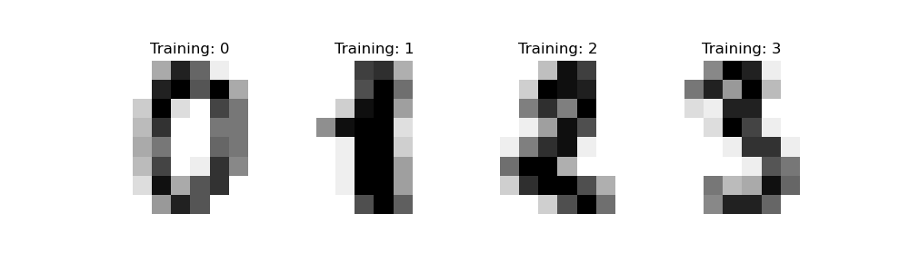
MNIST dataset consist of images of handwritten digits. Each images is of dimension 28×28 and there are 6000 of them in the set. The image is represented as a 2D matrix. So the complete dimension will be 28x28x6000.

Importing Neural net layers from Keras

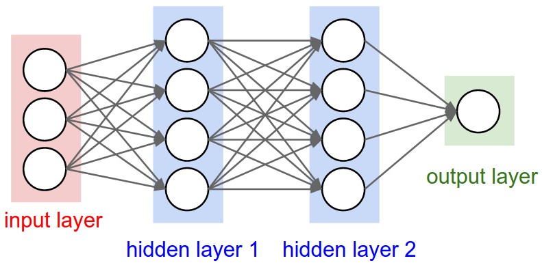
The convnet we are developing is similar to above picture. We need to import the layers from keras. If we were building it in pure python we need to build each layer from scratch. But keras comes preloaded with all the required layers. We are importing  Dense layer, Convolution layer(2D) , Max pooling layer ,Dropout layer

%matplotlib inline
import matplotlib.pyplot as plt
import numpy as np np.random.seed(923)
import keras from keras.datasets
import mnist from keras.models
import Sequential
from keras.layers.core import Dense,Dropout,Activation,Flatten
from keras.layers.convolutional import Convolution2D, MaxPooling2D
from keras.utils import np_utils
 

 

Setting up sizes

Here I am setting batch size as 128. That is the backpropagation algorithm will run as batches of size 128 each.

nb_classes variable is the number of classes that the dataset images belongs to. The neural net must predict one of these classes at the end if an image of a digit is given as input. Since our problem is to predict the digit , there are 10 classes (0-9)

image dimensions are set as 28×28. Since the images are represented as rows and cols in matrix we set img_rows and img_cols variable as 28

batch_size = 128

nb_classes = 10 # for 10 digits

#input image dimensions

img_rows , img_cols = 28,28

Loading the data

Now lets load the data. As i said earlier the data of images are in matrix form. We need to split the dataset to 2 types.

1. Training data
2. Testing data

Training Data

This is used to train our models. We define two variables X_train and y_train. X_train  will have the image matrix and y_train will have corresponding digit class

Testing data

This is used to test accuracy of our model.We have two variables for that as well. X_test,y_test

# load the data,
(X_train, y_train) , (X_test,y_test) = mnist.load_data()

If you are using spyder ide then variable explorer can be used to view the X_test and y_test variables.

Adding channel information

Here the dimension of the image right now is 6000x28x28. This does not have the channel information of the image.Color images have channel information for (R,G,B). Here we are reshaping the image matrix to add the channel information. This is required because the library function is expecting it. If we don’t add that information it may cause error. Since our images do not have color lets add 1 as channel .

channel first and channel last

The number of channels can be set in two orders in Keras. Either the channel number is given before the rows and cols information or we can give it at the end. This order can be configured in keras backend.

Kera stores all these configuration in a json file. In linux its stored in

$HOME/.keras/keras.json

NOTE for Windows Users: Please replace $HOME with %USERPROFILE%.

The default configuration file looks like this:

{
    "image_data_format": "channels_last",
    "epsilon": 1e-07,
    "floatx": "float32",
    "backend": "tensorflow"
}

Here we can set the backend for Keras to use. Either tensorflow or CNTK or Theano. The image_data_format is what we are interested in now. It specifies the order in which we must set the dimensions of input images. channels_last means the channel info is given at the end , channels_first means the opposite.

if K.image_data_format() == 'channels_first':
X_train = X_train.reshape(X_train.shape[0], 1, img_rows, img_cols)
X_test = X_test.reshape(X_test.shape[0], 1, img_rows, img_cols)
input_shape = (1, img_rows, img_cols)
else:
X_train = X_train.reshape(X_train.shape[0], img_rows, img_cols, 1)
X_test = X_test.reshape(X_test.shape[0], img_rows, img_cols, 1)
input_shape = (img_rows, img_cols, 1)

Categorize the classes

Each digit belongs to a class from 0 to 9. But our Neural network cannot understand the classes as a digit. This kind of data is categorical data. We need to categorize this 10 classes. To do that we make 10 columns .each indicating one of the classes. If an image belongs to a particular task our model sets one to that particular column.

To categorize the data , Keras provides to_categorical function

#categorize 
Y_train = np_utils.to_categorical(y_train,nb_classes) 
Y_test = np_utils.to_categorical(y_test,nb_classes)

Creating the model

Now all the preprocessing is complete. Let’s start to build our model. Keras provides layers class with all standard layers we need to create a convolution network

 model =Sequential()
 model.add(Convolution2D(6,5,5,input_shape =input_shape,border_mode='same'))
 model.add(Activation('relu')) 
 model.add(MaxPooling2D(pool_size=(2,2))
 model.add(Convolution2D(16,5,5,border_mode='same'))
 model.add(Activation('relu'))
 model.add(MaxPooling2D(pool_size=(2,2)))
 model.add(Convolution2D(120,5,5,border_mode='same'))
 model.add(Activation('relu'))
 model.add(Dropout(0.25))
 model.add(Flatten())
 model.add(Dense(84))
 model.add(Activation ('relu'))
 model.add(Dropout(.5))
 model.add(Dense(10))
 model.add(Activation('softmax'))

Sequential() object is initialized to create a sequential model. add() function is used to stack new layers to the sequential model

model.add(Convolution2D(6,5,5,input_shape =input_shape,border_mode=’same’))

• We are using 6, 5×5 filters in this convolution layer. That’s the first 3 parameters.
• input_shape is the dimension of images given as input.In keras we only need to give the input size for the first layer.All other layers can automatically find the dimensions.
• border_mode =’same’ sets all images to be of same size.More info can be found here

model.add(Activation(‘relu’))

• This is an activation Layer. The activation function is ‘Relu‘. We are also using a ‘softmax’ function at the end of our model.

model.add(MaxPooling2D(pool_size=(2,2))

• This is a  max pooling layer of size (2×2).

model.add(Dense(10))

• Dense layer is a fully connected layer in Keras.

 

Compiling the model

Till now we have designed our model. We have not yet compiled it.

 model.compile(loss='categorical_crossentropy',optimizer='adadelta')

We need to use compile() function to compile the model. We are giving the loss function and optimizer algorithm as parameters. ‘categorical_crossentropy‘ is used here as the loss function. ‘adadelta‘ is used for backpropogation.

 

Fitting the model

Once compilation is done , the next step is to fit the model. Here the fit() function is used in keras. We need to give the training(X_train,Y_train) data, batch_size, number of epochs and test data(X_test,Y_test) as input

 model.fit(X_train,Y_train,batch_size=batch_size,epochs=nb_epoch,verbose=1,validation_data=(X_test,Y_test))

This is the output.we can see the model getting trained.

Evaluation of our model

Our model is complete and is trained. Let’s try to valuate it.

score = model.evaluate(X_test,Y_test,verbose=0)

evaluate() function produces a score for our prediction

Prediction

res =model.predict_classes(X_test[:9])

Now our model is complete. We can now predict a handwritten digit image using our model. predict_classes() function is used to predict. The output is plotted as above.
Final code
#!/usr/bin/env python2
# -*- coding: utf-8 -*-
"""
Created on Tue Nov 21 08:16:25 2017

@author: akshaynathr
"""

%matplotlib inline
import matplotlib.pyplot as plt
import numpy as np
np.random.seed(123)

import keras
from keras.datasets import mnist
from keras.models import Sequential
from keras.layers.core import Dense,Dropout,Activation,Flatten
from keras.layers.convolutional import Convolution2D, MaxPooling2D
from keras.utils import np_utils
import keras.backend as K
batch_size = 128
nb_classes = 10 # for 10 digits

#input image dimensions
img_rows , img_cols = 28,28

# load the data,
(X_train, y_train) , (X_test,y_test) = mnist.load_data()

if K.image_data_format() == 'channels_first':
X_train = X_train.reshape(X_train.shape[0], 1, img_rows, img_cols)
X_test = X_test.reshape(X_test.shape[0], 1, img_rows, img_cols)
input_shape = (1, img_rows, img_cols)
else:
X_train = X_train.reshape(X_train.shape[0], img_rows, img_cols, 1)
X_test = X_test.reshape(X_test.shape[0], img_rows, img_cols, 1)
input_shape = (img_rows, img_cols, 1)
X_train /= 255
X_test /= 255

print("X_train shape:" , X_train.shape)
print("X_test_shape:" , X_test.shape)

#categorize
Y_train = np_utils.to_categorical(y_train,nb_classes)
Y_test = np_utils.to_categorical(y_test,nb_classes)

print("One hot encoding: {}".format(Y_train[0,:]))

for i in range(9):
plt.subplot(3,3,i+1)
plt.imshow(X_train[i,0], cmap ='gray')
plt.axis('off')

model =Sequential()
model.add(Convolution2D(6,5,5,input_shape =input_shape,border_mode='same'))
model.add(Activation('relu'))
model.add(MaxPooling2D(pool_size=(2,2)))
model.add(Convolution2D(16,5,5,border_mode='same'))
model.add(Activation('relu'))
model.add(MaxPooling2D(pool_size=(2,2)))
model.add(Convolution2D(120,5,5,border_mode='same'))
model.add(Activation('relu'))
model.add(Dropout(0.25))

model.add(Flatten())
model.add(Dense(84))
model.add(Activation ('relu'))
model.add(Dropout(.5))
model.add(Dense(10))
model.add(Activation('softmax'))

model.compile(loss='categorical_crossentropy',optimizer='adadelta')

nb_epoch =2
model.fit(X_train,Y_train,batch_size=batch_size,epochs=nb_epoch,verbose=1,validation_data=(X_test,Y_test))
score = model.evaluate(X_test,Y_test,verbose=0)
score
print("Test score:",score[0])
print("Test accuracy",score[1])

res =model.predict_classes(X_test[:9])
plt.figure(figsize=(10,10))

for i in range(9):
    plt.subplot(3,3,i+1)
    plt.imshow(X_test[i,0],cmap='gray')
    plt.gca().get_xaxis().set_ticks([])
    plt.gca().get_yaxis().set_ticks([])
    plt.ylabel("prediction=%d" % res[i],fontsize =10)