Building an AI Agent That Models in Blender: What Worked, What Didn’t

An experiment in letting an LLM drive Blender , a chat panel, a Python agent service, 700 viewport screenshots, and a lot of lessons about agent architecture.


Over a couple of weeks in March I built an experimental “Cursor for Blender“: a chat panel inside Blender where you type something like “create a wooden motorboat like this reference image”, attach a photo, and an AI agent writes and runs the Blender Python to build it, then looks at the viewport, judges its own work, and iterates.

This post is the honest version of how that went: the architecture, the three major rewrites, the results and what I’d do differently.

The setup

The system has two halves:

  • A Blender add-on: a chat UI in the 3D View sidebar, a scene extractor (objects, transforms, materials, relations), viewport capture, and a small execution layer that runs generated code in one undo group.
  • A local agent service: a Python WebSocket server that talks to an LLM (Claude, or any OpenAI-compatible endpoint). It receives the user message, the scene snapshot, and a viewport screenshot; it returns plans and bpy Python code.

The key feedback trick: every time code runs, the add-on captures the viewport and sends it back to the agent. The agent literally sees what it built. Over eight days of experiments the agent looked at the scene 697 times, every one of those screenshots is saved in a debug folder, which is why I can show you exactly what it saw below.

Iteration 1: tool calls (too rigid)

The first working version didn’t generate code at all. The LLM returned a JSON plan of whitelisted tool steps : create_primitive, move_object, add_light, set_material_slot, which the add-on validated and executed.

This was safe and predictable, and it could handle “add a sun light” or “move the cube up”. It could not build a boat. A dozen primitive-manipulation tools is nowhere near expressive enough for real modeling, and every new capability meant hand-writing another tool. The ceiling was obvious within a day.

Iteration 2: let it write Python, let it see

The second version gave the model two big upgrades:

  1. Python mode : instead of tool steps, the LLM writes a full bpy script and the add-on executes it.
  2. Vision : the viewport screenshot and user reference images go into every LLM call (this is when I switched to Claude for multimodal).

This is where it started actually modeling. Given this reference image:

Reference image of a wooden motorboat
The reference image given to the agent.

…the first attempts produced things like this:

First boat attempt — a crude, tugboat-like shape
Early attempt. The agent’s own quality-check verdict, visible in the panel: “The current model is a crude placeholder.”

Recognizably a boat. Not recognizably the boat. And single-shot generation had a fundamental problem: one giant script either mostly worked or failed halfway through, leaving debris in the scene the model didn’t know about.

Iteration 3: the “agentic” pipeline

So I built the thing everyone builds next: a multi-stage pipeline.

The final pipeline looked like this:

user message + reference images + viewport
-> intent extraction (LLM call 1)
-> image analysis (LLM call 2)
-> prompt refinement (LLM call 3)
-> detailed plan, up to 12 steps (LLM call 4)
-> per-step code generation (LLM call 5..N)
-> execute step in Blender
-> screenshot
-> strict quality gate (another LLM call)
-> satisfied? next step : refine / repair

Some genuinely good ideas landed here:

  • Incremental code generation. Code for step N+1 is only generated after step N has executed, using a fresh screenshot and scene snapshot — so each step sees reality, not the plan’s assumptions.
  • Error self-repair. When bpy code threw, the error, the failed code, and the live scene state went back to the model for a corrected version. Failed errors were also appended to a persistent log that got injected into future prompts, so the agent stopped repeating known mistakes.
  • Version-aware context. The add-on shipped the actual bpy API names and shader node types from the running Blender to the agent.

That last one mattered more than expected. My favorite failure: the agent kept using ShaderNodeTexMusgrave for terrain materials, a node that Blender removed in 4.1. You can see the error caught live in the panel here, mid-castle-build:

Castle with materials applied and a ShaderNodeTexMusgrave error visible in the panel
“Error: Node type ShaderNodeTexMusgrave undefined“: the model’s training data knows a Blender that no longer exists. It fixed itself after the repair loop fed the error back.

The results

The boat, over successive sessions, went from the crude placeholder above, through an over-stretched hull with furniture-like white blocks:

Mid iteration — elongated hull with white block seating
Mid-way: the proportions are off and the details are literal boxes, but there’s a hull, a deck, and seating in roughly the right places.

…to something with an actual hull shape, windshield, and wood materials:

Later iteration — recognizable motorboat with windshield and wood material
Later session: curved hull, windshield, seats, wooden deck. Still stylized, but clearly derived from the reference.

Here’s the step-by-step pipeline at work — the panel on the right shows the plan (“Step 3 of 9”), with code being generated for the next step from a fresh top-down look at the scene:

Top view of boat mid-build with the step list visible in the panel
Incremental mode: apply a step, look, generate the next one.

The castle was the more ambitious test: “Create a model like the Hogwarts castle. Use the reference image.” First pass, blocky:

First castle pass — blocky towers

After iterations of “add details” it became a genuinely respectable clay model, towers, spires, courtyard walls, a rocky base:

Clay-render style castle with many towers and spires
This is the moment the project felt like it worked.

What didn’t work

I want to be honest about the failure modes, because they’re more instructive than the successes.

The quality gate churned. I gave the verifier a strict prompt: results must be “detailed and real-life accurate”, with up to 6 refinement attempts per step. The session logs are full of Step 0: not satisfying, advancing to step 1/8, eight steps in a row where the judge never once said yes. A judge that demands photorealism from procedurally-generated primitives always says no, so its signal carried almost no information. Some sessions ended in failed after 3 attempts with the scene half-modified.

The pipeline lost context at every seam. Each of those 5+ LLM calls per turn was stateless, connected only by truncated text summaries of what earlier calls decided. The step-code generator couldn’t see the code from previous steps, only their titles, so step 3 had to guess what step 2 named its objects. Repairs happened on top of half-executed scripts, so the scene accumulated debris from failed attempts.

JSON was the wrong transport for code. Returning Python inside a JSON string field caused endless escaping bugs (a backslash-n arriving as a literal two-character sequence instead of a newline), which I patched with heuristics in two places. The codebase grew five separate “strip the markdown fence and parse JSON” functions.

Fail-open defaults lied to me. When the quality check returned malformed JSON, the code treated it as “satisfied” to avoid infinite loops — meaning a garbled response silently reported success. Debugging “why did it stop early” took longer than any modeling problem.

And costs multiplied. Every stage re-uploaded the viewport plus up to 8 reference images. One user message could mean five vision calls before the first line of code ran.

What I learned

  1. A pipeline is not an agent. Every hardcoded stage, intent extraction, prompt refinement, planning , replaces the model’s live reasoning with a frozen, lossy approximation of it. The stages I added to make the system smarter mostly made it forgetful.
  2. The feedback loop is the product. The single best design decision was making the agent look at the viewport after every change. The screenshots-plus-error-log loop is what took the castle from blocks to spires. Everything else was overhead around that loop.
  3. Judges need a relative bar, not an absolute one. “Does this satisfy what the user asked for” works. “Is this photorealistic” makes a judge that always fails you.
  4. Give the model ground truth, not vibes. A structured scene diff (what objects appeared, moved, changed material) after each execution would have been cheaper and more reliable than a vision call. That’s the top of my list for the rebuild.
  5. Version-pin the model’s world. LLMs know a Blender from their training data. Shipping the live API surface (and errors) into context fixed a whole class of failures.

What’s next

The rebuild is a much smaller system: one conversation, one tool-calling loop, run_python(code), screenshot(), inspect_scene(query), done(), with full history, so planning, verification and repair are just turns in a conversation instead of separate subsystems. The Blender add-on shrinks to a thin executor. Less code, more model.

The experiment version, for all its flaws, built me a castle. I’m curious what the simpler one can do.


Built with Blender 4.x, Python, WebSockets, and Claude. The screenshots in this post are the actual images the agent received during its runs, its point of view, unedited.

What if the universe is just boxes passing numbers around? (a weekend experiment)

A dust of thousands of small bright particles on a dark background, with a zoomed inset

Disclaimer up front: this is just an experiment , a toy model and a curiosity project, not a theory of anything. I am not claiming to have discovered new physics. I’m claiming to have had a lot of fun watching a grid of numbers misbehave.

Every once in a while a question gets stuck in my head and refuses to leave. This time it was:

If space were made of tiny discrete cells , little boxes that each hold some “excitation” and can only trade it with their neighbors , what would naturally emerge?

Not “can we reproduce electrons.” Nothing that ambitious. Just: start from almost nothing, and see what shows up uninvited.

The rules of my toy universe are deliberately minimal:

  1. Space is a 2D grid of cells.
  2. Each cell holds a number (excitation), between 0 and some maximum capacity.
  3. Cells only interact with their immediate neighbors. No action at a distance.
  4. Excitation is never created or destroyed , only moved around.
  5. Each timestep, every cell exchanges some excitation with its neighbors according to a rule.

That’s it. The exchange rule itself is the experiment: I don’t know what the “right” one is, so the whole point is to try many and watch.

The interpretation I’m chasing: if a blob of excitation forms that keeps itself together while stuff continuously flows through it, a stable attractor, then that blob is, in this toy universe, a “particle.” The pattern is the particle. Whether such things exist at all was question number one.

Building the lab

To explore this properly I built a small desktop lab in Python (NumPy for the engine, PySide6 + PyQtGraph for the interface, with Claude Code doing a lot of the heavy lifting). It has a live heatmap of the lattice, a formula editor where I can literally type an exchange rule as an equation and hot-swap the physics while the simulation runs, automatic detection of structures (it tracks them with IDs and tells me if they’re stable, growing, moving…), and a big number at the bottom showing total excitation every fram, because axiom 4 is sacred, and the software is built so that any rule I type conserves the total exactly. If a “particle” shows up, I want to be sure it’s physics and not a leaky float.

Then I started running experiments. Here’s what the universe did.

Finding 1: my universe froze solid

First serious rule: excitation is attracted to excited neighbors (transfer grows with how much the destination already has). I expected clumps. I got clumps, thousands of them, one or two pixels each and then absolutely nothing, forever. Every structure reported “stable,” lifetime 19,000 steps, velocity 0.000.

The reason is embarrassingly simple once you see it: in that rule, the flow between two cells is proportional to both of their excitations. So the moment a cell drains to zero, it becomes a perfect insulator, nothing flows in (transfer is proportional to its excitation, which is 0), nothing flows out (it has nothing). The empty cells wall off every clump from every other clump, and the whole universe locks into a frozen glass. Not particles. A parking lot.

A 256x256 lattice frozen into a static labyrinth of excitation, with a zoomed inset
5,000 steps in, and not a single cell will ever change again. The zoom shows why: every bright cluster is walled off by empty cells that conduct nothing.

Lesson one: a universe can die of stubbornness.

Finding 2: my “fix” was secretly just diffusion

Obvious fix: add a small leak, so empty cells conduct a little. I also simplified the attraction term to k * source * target * (max – target). Ran it. Everything dissolved into a smooth, boring fog. I turned the attraction knob k up 10x. Still fog.

Three snapshots showing lattice noise smoothing into a featureless fog
Crank k as high as you like, the “attraction” rule irons every wrinkle flat anyway.

Turns out this wasn’t a tuning problem, it was a theorem hiding in plain sight. If you compute the net flow between two neighboring cells A and B under that rule, the symmetric part cancels and you get: net flow = (A – B) * (k*A*B + leak). Always downhill. Always. The rule I thought was “attraction” was just diffusion wearing a costume. No value of k can ever make it clump.

The real requirement is an asymmetry: the transfer must depend on the destination more strongly than the source. Change target to target squared and suddenly excitation genuinely flows uphill toward concentrations. One character in the formula is the difference between fog and structure.

Lesson two: you can stare at an equation for a while and completely miss that it’s the same equation you were trying to escape.

Finding 3: 12,509 tiny particles

With the corrected rule, k * source * target^2 * (max – target) + 0.02 * source , the noise condensed into about 12,500 tiny bright spots sitting in a dilute background. And here’s the part that made me sit up: I ran it for 60,000 more steps and the count stayed at exactly 12,509. Nothing merged. Nothing evaporated. Each spot is a little standing balance: attraction pulling excitation in, leak bleeding it back out.

A dust of thousands of small bright particles on a dark background, with a zoomed inset
The census: 12,509 particles. I checked again 60,000 steps later, still 12,509. Not one merger, not one death.

By my own definition, these are particles: stable, localized attractors that persist while excitation continuously flows through them. They’re tiny (one or two cells) and admittedly a bit dull, which brings up the obvious next question.

Finding 4: getting anything to move is hard

Stable particles: check. But real physics has things that go places. So, can anything move here?

First attempt: shake the universe. I added noise to the rule, hoping the spots would random-walk like dust grains. Result: additive noise just evaporated them (it’s an extra leak in disguise , see Lesson Two, apparently I never learn), and gentler multiplicative noise left them alive but pinned to the grid, a spot drifted 0.27 cells in 20,000 steps. These particles are welded to the lattice.

What actually moves is something completely different: waves. With a threshold rule, cells hold their excitation until they exceed a trigger level, then discharge violently into their neighbors, a uniform background becomes fuel. Poke it, and a front races across the lattice, consuming the smooth background ahead of it. And because excitation is conserved, the burned fuel can’t disappear: it gets left behind as a churned-up, crystallized wake that can’t burn twice. I measured fronts traveling 40+ cells. And if you make the initial poke asymmetric (a dab of excitation next to an erased trench), the wave launches in one direction, like it knows where it’s going.

Four frames of a wave front sweeping left to right across the lattice
One poke (top), and the front sweeps rightward through the fuel, leaving crystallized ash behind.
Animation of the traveling wave consuming the background
The same wave, animated. I could watch this for an unreasonable amount of time.

So in this toy universe, matter comes in two kinds so far: frozen residents (the pixel particles) and travelers that burn fuel and die (the waves). Nothing yet that both persists indefinitely and moves, no gliders. My suspicion, after all this, is that a lonely scalar field with nearest-neighbor rules simply can’t do it, and that persistent movers need either longer-range sensing or a second quantity per cell (something momentum-like). Which would be a satisfying outcome in itself: the model telling me what it’s missing, instead of me assuming it upfront.

What’s next

The queue: do these particles survive on hexagonal grids, or are they square-lattice artifacts? Can two waves collide and do something interesting? Can two particles ever bind? And the big one, introducing a second variable per cell, but only because the experiments above demand it, not because I want it.

Once more for the people in the back: this is just an experiment. A toy universe on a 256×256 grid, made of five assumptions and a formula box. But there’s something genuinely addictive about typing an equation, pressing Run, and finding out your universe froze, dissolved, crystallized into 12,509 specks, or caught fire and burned across the screen, none of which I asked for. That’s the whole appeal of emergence: you write the rules, and the consequences are still a surprise.

Happy new year. Hello RL

Happy new year everyone. A fantastic new year is here. Wishing everyone a great year ahead.

As I mentioned in the title, I am planning to study Reinforcement learning this year. For the last two years, I have concentrated on machine learning algorithms mainly related to Deep neural networks. Starting with Andrew Ng’s CS 229 in 2017, it has been a great journey so far.

2019 is the year of Reinforcement -learning

I have been following a lot of recent research papers and many of them are having a mixture of Deep learning models and Reinforcement techniques. This is a strong indication that 2019 in the year of reinforcement learning.

What is Reinforcement learning?

In reinforcement learning, we are training an agent in an environment. Each action of the agent gives a positive reward or negative reward. The goal of the agent is to maximize the reward.

Diagram of reinforcement learning process

Google beat the best Go player with AlphaGo using a combination of techniques that involves reinforcement learning(Deep Reinforcement Learning).

Uber recently solved Montezuma’s Revenge by Go-Explore

Image result for Montezuma’s Revenge
Montezuma’s Revenge Game

The biggest advantage is that we can combine the Deep learning networks and Reinforcement learning techniques together to create really powerful algorithms.

Plan of Study

I have gone through some basic understanding of RL last year in the following lectures:

[UC Berkeley] CS188 Artificial Intelligence by Pieter Abbeel

[Stanford] CS229 Machine Learning – Lecture 16: Reinforcement Learning by Andrew Ng

I watched these lectures long time back and since I was concentrating more on Deep learning , I did not follow up much on RL. So I am planning to start with the following Lecture series:

Deep learning Bootcamp :https://sites.google.com/view/deep-rl-bootcamp/labs

I am thinking of writing a blog for each of the lectures and labs associated with it.

That’s all for this blog. If you are also starting RL this new year let me know about it in the comments.

2018 coming to an end

It is December again. Another wonderful year is coming to an end. It’s been a long time since I posted my last blog here. Was extremely busy with my job at Oracle. Even though I was very busy I managed to do some good work in Deep learning.

Courses

In the last 5 months, I completed some  great courses from Coursera and Youtube on Deep learning.

Deeplearning.ai is one of the courses I did in the last 5 months. This is a package of 5 courses starting from Basics of the Neural net to Advanced concepts like CNN, RNN, GRU, LSTM etc. It costs about 3000Rs per month for subscribing to the course and will take nearly 3-4 months to complete. Working through this course I am able to understand and implement most of the latest concepts in Deep learning. This is an extremely recommended course for everyone who is interested to learn advanced concepts.

Deep learning Frameworks

I am able to work on some deep learning frameworks including TensorFlow, PyTorch and Keras. I also did a course in datacamp to learn more about Numpy.

Kaggle

Image result for kaggle

I finally started to participate in Kaggle competitions. I heard about kaggle for the first time about 2 years back. I recently participated in the PUBG kernel competition to predict the chance of a player to win the game. Kaggle is more than just participating in competitions. There is a section known as Kaggle learn where there are free tutorials that teach from the basics of machine learning to Advanced concepts like CNN implementation. Many people share their Kernel which has extremely valuable information relating to the techniques, algorithms,implementation etc.

Learn Maths

I started to relearn the mathematical concepts like Probability ,Linear algebra and Vector calculus. I am currently going through my old college textbooks. Knowing these concepts really helps in understanding research papers with some heavy math.

Code

I have also worked on some code for ML algorithms that I learned and implemented. I have uploaded some of them in my GitHub repo

The following is an interview video with an ML PhD student. I particularly liked this because of the quality of discussion on GAN.So I am putting it here.


Word embedding and word2vec

Image result for word embeddings

In Natural language processing , word embeddings are extremely important. An efficient embedding can give extremely accurate results. Let’s discuss a little about word embedding in this post.

Introduction

Consider files like  images , sound files or video files. They contain a lot of information about the contents. For eg: a set of pixels in an image carries a lot of information and this relation can be useful for further analyzing patterns in that image. Same is applicable for sound files. It carries a lot of information like frequency , amplitude etc which can be correlated. These information can be efficiently represented in matrix form and the relationship between these characteristics are preserved.

But in the case of text , how can we efficiently represent them. How can we find the relationship between individual words and represent them efficiently without loosing this relation.

Language Models

Anything with text needs a language model.  Language model tells how individual words come together.

A language model computes the probability for a sequence of words P(w1 ……wT).

One-hot representation

One-hot representation is a vector representation for words . The words are represented in a vector format with all elements 0 and one element 1.

For ex: Consider this sentence : I love deeplearning.

I is represented by       –> [1 ,0 ,0]

love is represented by  –>  [0 , 1 , 0]

deeplearning  is represented by  –>  [0 , 0, 1]

We can see that the vector is a sparse vector

Problem: The issue with one hot vector representation is the length of the vector is equal to vocabulary.

Vocabulary is the set of all words that we consider. As the size of vocabulary increases the size of one-hot vector also increases.

How to preserve the relation between words?

As we can see, one hot vector do not extract any kind of relation between words. We need methods to extract this relation.

If we can reduce the dimension to a lower dimension , may be we can extract some relation. This is similar to the PCA( Principal component analysis). So based on this intuition let’s see the possible techniques  and  ideas.

Idea 1: Reduce Dimensionality

Image result for word embeddings

We can apply dimensionality reduction and map the words to a lower dimension. This way we can find the relationships.

Using SVD (singular value decomposition) of matrix we can reduce the dimensionality.

But this is not applicable to a large dataset since the complexity is quadratic.

Idea2: Find the vectors without matrix decomposition

Without using highly complex algorithms, we can find an approximation of the lower dimensional matrix. This idea is based on the following hypothesis.

Distribution hypothesis

“Words that are used and occur in the same context tend to support similar meaning”

Surrounding words of a center word has same meaningful relation with that of the center word.

Vector for word representation : word2vec and Glove

word2vec ,Glove etc are vector word representations that learn relationship between words.

Outputs of these representations are words with interesting relationships as below

  vec(King) -vec(man) + vec(women)   =  vec(queen)

Word2vec

Let’s dig in more into word2vec. word2vec consists of two algorithms

  1. CBOW(Continuous bag of words)
  2. Skipgram

CBOW predicts the center word from the context words

Skipgram predicts the context words given the center word.

CBOW (Continuos Bag of words)

Image result for cbow

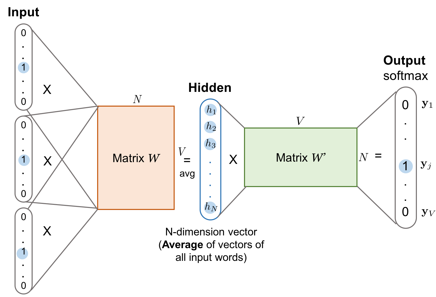
CBOW predicts the center word when the context words are given as input. In CBOW a neural net is used to approximate the context word matrix.

Center word and context words.

Related image

In the first step we define a window size. The window size is the number of words we consider. For example in the above picture the window size is set as 2.

window size  is a hyper parameter.

So 2 words on either side are taken. The blue colored word is the center word and the surrounding words in the window are context words.

Image result for cbow

We can see above how the training data and labels are created. Here the window size is set as 1 in above picture. (Note:Both pictures above are completely different projects)

CBOW formula deduction

Image result for cbow

To make it easy for us to deduce the formula for the CBOW , lets consider a simple model with only one word in the context as input.

The input x

x is a one-hot representation vector, which means for a given input context word, only one out of V

V units, {x1,⋯,xV}

{x1,⋯,xV}, will be 1, and all other units are 0. for example,

x=[0,⋯,1,⋯,0]

x=[0,⋯,1,⋯,0]

The weight between the input layer and the output layer can be represented by a V×N matrix W. Each row of W is the N-dimension vector representation Vw of the associated word of the input layer.


Selection_012


So we have found the probability of the context words using the softmax function.  We need to define a cost function so that we can maximize the proabability. We can use   log-likelihood to maximize this.

In the next post , lets discuss more about the cost function and the mathematical steps to derive updates.

We will also discuss about skipgram model and will deduce the probability and cost function and finally we will look at how these two algorithms work in word2vec.


What is learning in ML algorithms.

downloadMachine learning is a big trend in the industry now. The performance of these algorithms are improving every day and coming in par with human skills.

A machine learning algorithm is an algorithm that learns from data. But what does it really mean by ‘learning’. How can we define it accurately.Only something that is defined can be analysed and measured right.

In the book (‘Machine Learning’ by Tom Mitchell (1997))  , learning is defined as follows

A computer program is said to learn from experience E    w.r.t  some class of task T and performance measure P, if its performance at tasks in T, as measured by P, improves with experience E.


Xavier Initialization

I was reading code implementations of various GAN models and something very beautiful struck me. It was a very simple function used in all of those implementations called “Xavier Initialization”.

After some digging up in google I found out that its something worth writing for today. I have heard about Xavier initialization first in  cs234n lecture by Stanford. I didn’t search for it then, but today I have finally found it.

So what’s it?

Xavier Initialization is a method used to initialize neurons in Deep learning networks. When we start to model deep neural nets , the initialization values are always confusing. Proper initialization can get your network converged faster or getting stuck.

  • If the range of values are small then it might not reach deep into the network because it can fade away.
  • If the initial values are large then it might reach at the end with massive values which make it useless.

Xavier’s method of initialization take away these problems by  initializing the weights in network from a distribution with zero mean and a specific variance,

\text{Var}(W) = \frac{1}{n_\text{in}}

How it works?

As I said earlier, the Xavier’s method keeps the variance in all layers same. Let’s assume the neural network as

Y = W_1X_1 + W_2X_2 + \dotsb + W_n X_n

Let’s take the variance

Var(y) =Var(w1x1 + w2x2 + … + wNxN + b)

Since b is a constant ,its variance turns out to be 0


Note:If two variables are independent we can write the variance as below

{\begin{aligned}\operatorname {Var} (XY)&=[E(X)]^{2}\operatorname {Var} (Y)+[E(Y)]^{2}\operatorname {Var} (X)+\operatorname {Var} (X)\operatorname {Var} (Y).\end{aligned}}

Here E() is the Expectation. If the weights are from a Gaussian distribution , the mean is zero. So E() terms turn out to be zero.

\text{Var}(W_iX_i) = E[X_i]^2 \text{Var}(W_i) + E[W_i]^2 \text{Var}(X_i) + \text{Var}(W_i)\text{Var}(i_i)


\text{Var}(W_iX_i) = \text{Var}(W_i)\text{Var}(X_i)


substituting this equation we get,

\text{Var}(Y) = \text{Var}(W_1X_1 + W_2X_2 + \dotsb + W_n X_n)


If we assume that X and W are independent and distributed identically then,

\text{Var}(Y) = \text{Var}(W_1X_1 + W_2X_2 + \dotsb + W_n X_n) = n\text{Var}(W_i)\text{Var}(X_i)


Var(Y) is variance of output.  Var(X) is variance of input. From above equation it turns out that variance of output is   n*Var(W) times scaled value of variance of input.


To make the variance of output and input the same  n*Var(w) must be equal to 1.

\text{Var}(W_i) = \frac{1}{n} = \frac{1}{n_\text{in}}


Xavier initialization in Frameworks


Tensorflow

W = tf.get_variable("W", shape=[784, 256],
           initializer=tf.contrib.layers.xavier_initializer())

Caffe

weight_filler { type: "xavier" }

GAN -Generative Adversarial Network

“(GANs), and the variations that are now being proposed is the most interesting idea in the last 10 years in ML”

These are the words of Yann LeCun, one of the very famous researchers in Deep Learning. GAN or Generative Adversarial Network is considered to be one the most promising developments in ML last year.

What is GAN?

If you have some idea about deep learning networks you will know about using them for various tasks like NLP, image recognition, object detection etc. Neural networks work extremely well in all these tasks. But does it mean it can do well in all areas? Imagine this situation. An artist is creating a masterpiece drawing. A neural network might be able to recognize objects in the image, but can we create a network which can create a great painting like that. Can a machine write beautiful articles and publish them. This is considered to be of great difficulty since we train the networks with existing data. The problem here is to make the network generate its own data. This is a Generative task.

The issue with the Generative task.

Imagine you are learning chess. If you want to improve your game you need a powerful opponent who does innovative moves. A chess player improves his game skills by analyzing his moves and finding the mistakes. If we are creating a model for chess we train it using many moves we manually prepare.

Image Generation Problem.

Image generation problem is where the machine learning model generates an image by itself. Imagine a machine creating a drawing as beautiful as Picasso. We give a set of images for training and the model generates the image while testing that it is similar to the training images, but are not same.

Problem

Here the issue is that we need a way to score the output image. If there are 2 output images, how can we say which one is better?

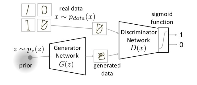
GAN proposes to use a neural network for this process. So in addition to the model, there is another neural network that scores the image output. The neural net that generates the image is called Generator and the one that scores the image is called the Discriminator.


Working of GAN?

As I said earlier there are 2 neural nets basically. Generator and Discriminator.

Generator

The generator has the duty of generating a novel image based on the patterns in the training samples.It uses the probability distribution to generate the similar patterns of the test set in the output image. We can see Generator as the function G(z). It takes the input z which is the sample from the probability distribution p(z).

Discriminator

Discriminator takes input from two sources. Real data and generated data from Generator. Its duty is to score the images into classes – Generated, Real. i.e it tells whether the input image is a real image or a generated image. It uses a sigmoid classifier to score the images

Training GAN

Training of GAN is done similar to two agents, playing with each other in a reinforcement learning setup. Here, Generator is trying to create an image that is indistinguishable by Discriminator and Discriminator is trying to discriminate the image from the real image. Like a game right?

Mathematically it is represented as

In the function V(D, G), the first term is the entropy of log likelihood of sample data from Probability Distribution of real data. Discriminator tries to maximize this value to 1. The second term is the entropy of generated image(fake image). The discriminator tries to maximize this to 0.


Applications of GAN

1. Increasing resolution of Image

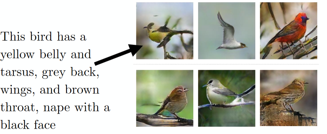
2. Text to image generation

This is implemented with some modifications called Conditional GAN. Paper

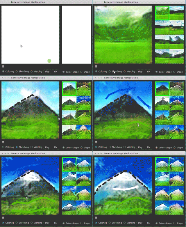
3. Interactive Image Generation

Conclusion

Here I have tried to give a simple and brief idea about GAN.In the next post, let’s look at training a GAN more practically and let’s implement one in tensorflow.

Happy new year

It’s 2018. Happy new year to everyone. Last year has been amazing. Many memories and learnings. Planning to make a lot of crazy adventures this year. New year resolution of this year is to blog every day about the stuff I learn in the field of Artificial intelligence, Computing, and Mathematics. I have found that when I blog about a particular topic I am understanding it a lot better. I am extremely excited about all the new things I am gonna learn this year.

Wishing everyone a crazy and exciting year ahead.

Learning Convex Optimization

https://web.stanford.edu/~boyd/cvxbook/bv_cvxbook_cover.jpg

Starting to learn a very new topic. After undergrad maths classes , its been a while since I learned any new maths concepts. After going through many lectures on ML and deep learning I find that most of the problems are optimization problems. That’s when I got introduced to Convex optimization. Found this amazing book. I will be going through the book along with lecture